|
Voxel
|
|
Voxel
|
Describes the algorithm used to infer surface normals from the depth buffer.
We estimate the normal vectors of all pixels on the screen by finding the gradient  of the depth buffer
  (in screen coordinates), and then using this gradient to calculate the normal vectors, according to the following equations:

Here,  is the 3D ray (in world coordinates) along which the pixel at the given coordinates was traced, so that
  is the coordinates of the intersection, and
  and
and  are those for the adjacent pixels in the horizontal and vertical directions, respectively, based on the gradient. The resulting normal vector
  is calculated using the vector cross product
  .
.
There are two main challenges, both having to do with how one finds the image gradient:
In order to address these issues, gradients are estimated using a MRF.
For the moment, forget about "depths" (which actually require a little bit of special handling), and imagine that  is just a function of which we want to find a smoothed boundary-respecting gradient. At every pixel, our MRF will attempt to estimate two quantities:
 , the smoothed value of .
 , the smoothed gradient of .
Assume that there is a Gaussian probability distribution over these quantities. The mean of this distribution is what is computed and stored for every pixel (that is, we perform something like expectation propagation), while the covariance is a fixed parameter to the model. To be more specific, and are derived from the neighbors of  as:
as:

Here, ![$\delta^{(i)}_{x,y}\in[0,1]$](form_15.png) is the "weight" assigned to the
is the "weight" assigned to the  th neighbor edge in the MRF. If it is zero, then this neighbor makes no contribution, and if it is one, then it makes a full contribution. Along occlusion boundaries,
  should be zero. The
  vectors indicate the relative positions of the neighbors. For example, for neighbors in the four cardinal directions, we may take
  and
and  for the neighbors which are up, right, down and left of the current pixel, respectively. The three terms making up the distribution have the following interpretations:
 , causes the smoothed value to be close to the observed value .
 , causes
  , which is what the smoothed value and gradient at indicate the th neighbor's value should be, to be close to the smoothed neighbor's value
  . This is, in a sense, the most important term, since it causes the smoothed values and gradients to be consistent with each other.
 , causes the smoothed gradient to be close to that of the neighbor,
  .
.To actually find and , we take logarithms, differentiate, and set the result equal to zero, yielding:

Notice that the second equation, resulting from differentiating with respect to , is two-dimensional. Hence, this is a  linear system, which can be solved (reasonably) efficiently using e.g. Gaussian elimination. In fact, simply computing the coefficients of the system (i.e. evaluating the above equations) is more expensive that solving it.
This gives us our "basic model": simply iterate over all pixels evaluating and solving the above linear system, and repeat until convergence (this will be refined in subsequent sections–see Optimizing and Coarse-to-fine). At this point, I should point out that we only store a state at each pixel, rather than a message for each edge in the MRF. One will often use a message-passing algorithm (e.g. belief propagation) to optimize a MRF, in which the message sent from pixel to the neighboring pixel  is based on all of the incoming messages to except that from . The reason that message passing is used is that the state of pixel should not depend on its state at an earlier iteration, and the state at depends on the the earlier state of , since these pixels are neighbors. Message passing removes these "first order dependencies", but other, longer dependencies still exist (e.g. to
  to )–it only gives a "correct" algorithm on a DAG (i.e. the model is a Bayesian network), which our MRF is not. I did experiment a little bit with message passing, but it is more computationally expensive than simply storing a state for each pixel (roughly four times so in a four-neighbor model), and didn't improve performance enough to justify the cost.
While we're on the subject of trade-offs, one may have noticed that I didn't talk too much about the edge weights . The "traditional" way to deal with occlusion boundaries, which I've encountered in stereo vision and image denoising algorithms, is to use latent variables. More precisely, one assumes that each edge has some probability  of being an occlusion boundary, and then modifies the distribution to be:

Where  is derived from and the normalization constants of the Gaussian distributions. It is possible to use this model, although solving for and in a four-neighbor model requires solving
  different linear systems (one for each term which results from multiplying out the above, not including the trivial
  term). Once more, this is simply too expensive. It is much better to choose the values of beforehand, using a heuristic (see Applying to a depth buffer).
I've already roughly described how we optimize the MRF: find the state for each pixel, and repeat until convergence. For version of the MRF which I most commonly use, the state of each pixel depends on the states of its neighbors in each of the four cardinal directions (see Coarse-to-fine for an example in which the neighbors are taken to be in the four diagonal directions). We could sequentially step through the screen in, say, row-major order, and update each pixel when we reach it. However, this model admits a large amount of parallelism, and we'd be foolish not to exploit it.
The simplest method for performing the updates in parallel is probably this: maintain two buffers, and update each pixel in parallel, reading the states of its neighbors from the first buffer, and writing the result to the second. After doing this for all pixels, simply go the other way, reading from the second, and writing to the first. The biggest advantage of this strategy is that will naturally tend to use coalesced memory accesses on GPUs which benefit from them. However, it has the disadvantage that information will propagate through the graph very slowly. When a pixel changes, only its neighbors will "be aware" of the change after one iteration, only their neighbors after two, and so on.
Addressing this problem by using a more sophisticated strategy is probably not advisable on a GPU. On a multi-core processor, however, we can benefit from using an in-place update, for which we keep only one copy of the states, and specify a mixed parallel/sequential updating strategy which both ensures that no thread will be writing to a memory location that another is reading, and causes imformation to propagate rapidly through the graph.
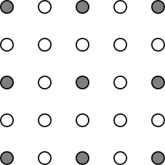
One such strategy is based on the idea of imagining that the graph is a checkerboard. We first update all of the black squares:
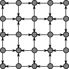
Here, the arrows point to the nodes which are being updated, from those on which they depend. Next, we update the white squares:
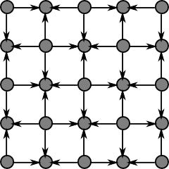
Alternation between the two continues until convergence. The computation of each black square does not depend on the result at any other black square, and likewise for the white squares. Hence, all squares of each color can be considered concurrently.
This is a reasonable "baseline" method, and will be the foundation of the coarse-to-fine updating strategy (see Coarse-to-fine). However, it is not the best. An alternative is to parallelize over the even-numbered rows, and, within each row, sequantially visit the pixels from left-to-right:
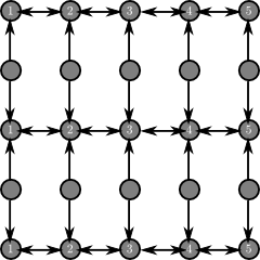
Here, the numbers within each row indicate the sequential order in which the updates are performed. We next update the odd-numbered rows:
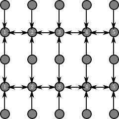
We then do to the same from top-to-bottom, right-to-left and bottom-to-top, updating each pixel a total of four times, once for each direction. This approach results in information potentially propagating all the way across the graph in a single pass (that is, a change to a pixel on the left side of the screen will affect a pixel on the right side), whereas after visiting all pixels four times in the "checkboard" order, information will have propagated a distance of at most eight pixels.
Of course, we need to have a model which not only gives high-quality results, but also one which can be optimized very quickly. The best way that I know of to speed up convergence is to perform the optimization in a coarse-to-fine manner.
Let  be a "coarseness level", and imagine that each node in the coarsened grid corresponds to a
  "block" of nodes in the finest grid (for which
  ). We will treat this block as a single node in the coarsened grid, with the corresponding data term being the value at the center of the block, and the probability distribution defining the update being modified to account for the change in scale.
Every edge in the coarsened grid corresponds to  edges in the finest grid, so we must raise the two smoothing terms of the distribution to the th power. Similarly, because there are
  nodes in each coarsened block, we must raise the data term to the th power. Because the centers of the blocks are times further apart, we must scale
  by a factor of . Finally, the variances of the two smoothness terms must be scaled, but it's unclear how this should be done–one could make a case for scaling by or , depending on whether we prefer to view the accumulated errors along a stretch of nodes as being independent (the former case) or identical (the latter). I use the former:

Finding the expectation of this distribution is essentially the same as before (see Basic model). The more difficult question is how one transitions from a coarser grid level to a finer one. The approach taken is as follows: starting from the following coarse grid (dark circles correspond to nodes which have been computed):
We begin by performing a diagonal update:
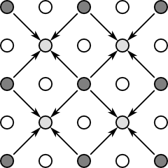
This is essentially the same as the "checkerboard" update, with the difference being that the neighbors, represented by , lie not in the four cardinal directions, but rather the four diagonal directions. We next perform a "checkboard" update in the cardinal directions:

At this point, the entire finer grid will be populated. The overall coarse-to-fine optimization procedure is to start at some predetermined coarseness level , perform some number of smoothing passes (see Optimizing), and then transition to level  using the procedure described above. We then repeat this until .
I mentioned earlier that applying this model to a depth buffer requires "special handling". The reason for this is that, in a depth buffer, the rays are diverging. If one considers a scene consisting of a single plane meeting the horizon, then although the plane itself is linear, the depth buffer will not be–close to the horizon, adjacent pixels will have very different depths, while far from the horizon, they will be much closer. Hence, we do not smooth depths, but rather reciprocal-depths, which do vary linearly when they correspond to the depths of a plane. One can derive the gradient  from
from  using the chain rule:
  . So, we smooth the reciprocal-depths, apply the chain rule to find the gradients of , and calculate the normal vectors.
The heuristic which I use to calculate is simple soft-thresholding of the difference between adjacent depths:
![\[ \delta^{(i)}_{x,y} = \max\left(0,\min\left(1,\frac{r_h - \left\vert f(x,y) - f(x+d^{(i)}_x,y+d^{(i)}_y) \right\vert}{r_h-r_l}\right)\right) \]](form_47.png)
If the depths differ by at most  , then
  , while
  if they differ by at least
  , with varying linearly in-between. The thresholds and are not constant–rather, they are based on the size
  of the voxels at the depth . For example, if we're drawing a
  scene (which lies in a
  cube), then
  . Due to mip-mapping, however, might be larger: the ray-casting routine performs mip-mapping in such a way that the smallest voxels are always at least one pixel in size when rendered, so
  , where is a proportionality constant measuring the size of a pixel, and depends on the screen resolution and field of view. I take the smallest which satisfies these two equations, and then define
  and
and  , where
  and
and  are parameters satisfying
  .
.
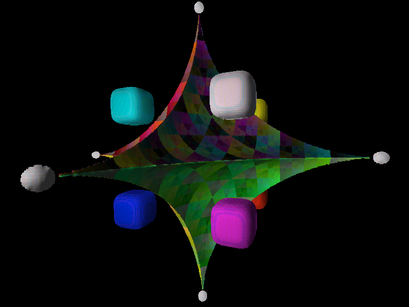
I'll conclude by including some screenshots which illustrate the various parts of this process, on a simple test scene containing a  voxel representation of a bunch of superquadrics. The first image shows the heuristically-found edges (see Applying to a depth buffer):
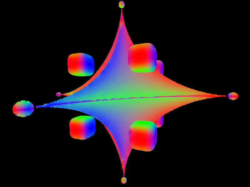
From the depths, optimizing the MRF (see Optimizing) and solving for the normal vectors (see Overview) gives the following result. Here, each color channel contains the magnitude of one component of the 3D normal vector:
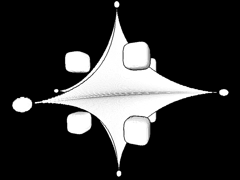
One can whip up some simple "fake" diffuse lighting by taking the illuminance at each pixel to be the positive part of the inner product of the normal vector with a vector pointing towards the light source:
 1.8.1.2

